Implementing a B-Tree in Go
The B-Tree is a self-balancing search tree data structure that allows for efficient insertion, deletion, and retrieval operations in logarithmic time while keeping all data in sorted order. B-Trees were developed by computer scientists Rudolf Bayer and Edward M. McCreight at Boeing Scientific Research Laboratories to solve the problem of organizing and maintaining indexes for on-disk files that are constantly changing, but need to be accessed randomly. They were introduced to the general public in 1970.
Today, the B-Tree is commonly used in databases and file systems to store and organize large amounts of data on secondary storage. As an on-disk data structure, B-Trees are designed to minimize the number of disk accesses required for insertion, retrieval, and deletion, making them an ideal choice for highly efficient and scalable data storage systems that process vast amounts of data.
Occasionally, B-Trees can also be useful as in-memory data structures because of the locality of reference when searching. B-Tree search operations can make efficient use of memory caching on modern processors and, in some cases, even outperform more conventional in-memory data structures such as red-black trees or AVL trees.
In today's article, we'll explore how B-Trees work by implementing a fully functional in-memory B-Tree in Go, providing insertion, deletion and retrieval operations. In a future article, we will expand on this version to also create a disk-resident B-Tree that dynamically stores and retrieves its nodes from secondary storage. But before that, it is crucial to understand how the in-memory version works, so let's dive right in!
B-Trees vs. Binary Search Trees
Let's go over our knowledge of trees in general.
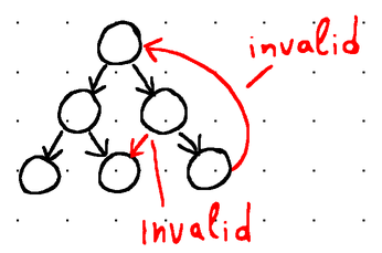
In computer science, a tree is just a collection of nodes that branch off of a single root node. Each node optionally contains a list of references to other nodes (its children) as well as some data, with the constraint that no reference can appear in the tree more than once (i.e., no two nodes can point to the very same node) and there can be no references to the root node.
For instance, the tree shown below is invalid, because a child node points to its root and two internal nodes point to the same child:
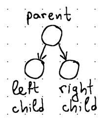
The maximum number of children that a node can have is called fanout. For instance, binary trees get their name from having a fanout of 2 (meaning each node in the tree can have no more than 2 children, usually called left child and right child).
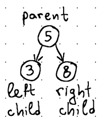
Each node usually stores some identifier (a key or a value of some sort) that can be used for sorting. We refer to a tree as a search tree when its nodes are maintained in sorted order. In binary search trees, for example, the left child value is always smaller and the right child value is larger than the value of their parent.
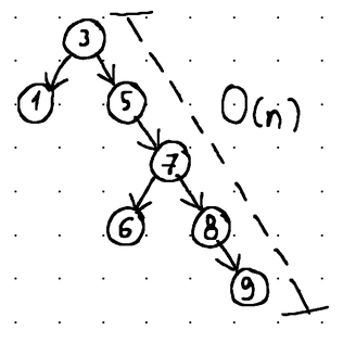
Lastly, we can distinguish between balanced and unbalanced binary search trees. A balanced tree is basically a tree in which the heights of the left and right subtrees of any node differ by no more than 1 (i.e., the overall height of a tree with N nodes leans towards log2N)
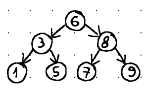
Put differently, balancing guarantees that insertion, deletion, and retrieval operations can be fulfilled in O(log n) time (with n being the total number of nodes in the tree). In contrast, operations in an unbalanced tree may degrade to O(n) time (linear time complexity):
The balance in a tree is maintained through rotations. Rotations alter the structure of the tree by completely rearranging the links between its nodes, while maintaining their sorted order and limiting the height difference between the right and the left subtree to a maximum of 1.
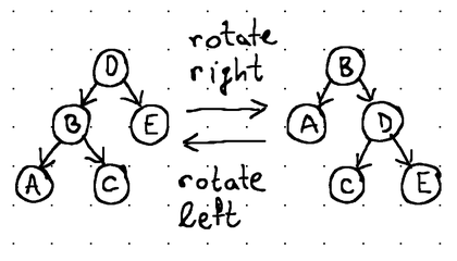
Rotations occur as nodes are added to and removed from the tree, and while balanced binary search trees are, without a doubt, very useful as in-memory data structures, these frequent rebalancing operations make them impractical for use with external storage.
Remember that with secondary storage, data is transferred to and from main memory in units called blocks. So, even if we just want to read or write a single byte of data, at least a few kilobytes of data are fetched from the underlying storage device into main memory to be updated and flushed back to disk.
A simple insertion or deletion usually causes multiple rotation operations to restore the balance, and this could sometimes drastically rearrange the entire tree, meaning we often have to rewrite large portions of its on-disk representation (if we are to persist it on secondary storage).
Furthermore, the low fanout means that the tree is usually quite tall, and assuming that every node resides at a different location on disk due to the constant rebalancing operations, traversing the tree to find a specific value may very likely require you to perform log N disk scans to retrieve data (N being the number of nodes in the tree).
Now imagine both scenarios with a disk-resident binary search tree of, say, 1 TiB in size. Having to scan 0.5 TiB on disk to find a simple value or to rewrite hundreds of gigabytes of data on disk just because an insertion rearranged most of the tree doesn't sound too good.
The main idea behind B-Trees is to solve both of these issues by increasing fanout, thus reducing the overall height of the tree and bringing both the child pointers and the data items closer together. With that, the same amount of information that would often be scattered across hundreds of binary search tree nodes can now be stored in a single B-Tree node. And since a B-Tree node is usually designed to occupy a full block of data on secondary storage, both insertion, deletion, and retrieval can usually be fulfilled in O(logfN) time instead of O(log2N) time (f being the fanout of the B-Tree, and N being the total number of data items in the tree).
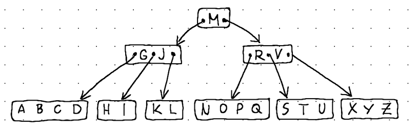
Other than that, a B-Tree is simply a balanced search tree.
B-Tree Variants
The original B-Tree has evolved over time and different variants exist today, with the B+-Tree and the B*-Tree arguably being the two most popular versions. We will touch on these two versions very briefly in order to contrast them to the B-Tree that we are going to implement in this article.
In a traditional B-Tree, every node contains raw data, plus keys and child pointers that can be used for navigation. In a B+-Tree, only the leaf nodes contain raw data, while the root node and the internal nodes only contain keys and child pointers that can be used for traversing the tree. In addition to that, the leaf nodes are linked to each other, forming either a singly or a doubly linked list, used for easier sequential scanning of all keys in ascending or descending order.
B*-Trees are often confused for B+-Trees, because they exhibit similar properties. However, in addition to the changes present in B+Trees, B*-Trees ensure that each node is at least 2/3 full (compared to 1/2 in B-Trees and B+-Trees) and they also delay split operations by using a local distribution technique that attempts to move keys from an overflowing node to its neighboring nodes before resorting to a split (we will discuss the split operation in greater detail later in this article when designing the insertion algorithm).
In today's article, we are going to implement a classical B-Tree, where keys, data items and child pointers all live together in the nodes of the tree.
B-Tree Anatomy
A B-Tree, like any other tree, is made up of nodes, and each node carries some data.
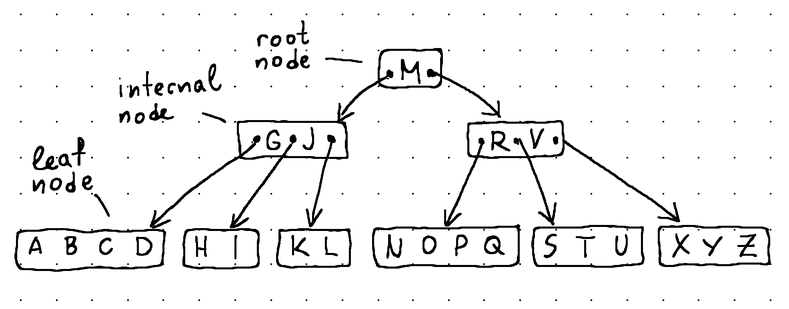
- The root node sits at the very top of the B-Tree and has no parents.
- The leaf nodes sit at the very bottom and have no children.
- The internal nodes (all other nodes in the tree) sit between the root node and the leaf nodes and usually span multiple levels. They contain both data and child pointers.
All nodes are subject to some constraints when it comes to the number of child pointers (if they are non-leaf nodes) and the number of data items they can store. They cannot go beyond a specified minimum and maximum threshold. These thresholds are determined by the degree of the B-Tree.
The degree is a positive integer that represents the minimum number of children a non-leaf node can point to. For instance, in a B-Tree with a degree of d, a non-leaf node can store no more than 2d and no less than d child pointers. The only exception to this rule is the root node, which is allowed to have as little as two children (or no children at all if it is a leaf). The minimum allowed degree is 2.
Additionally, a non-leaf node with N children is stated to always hold exactly N - 1 data items (by definition). These limits can easily be derived from the degree of the B-Tree by making the following calculations:
const (
	degree      = 5
	maxChildren = 2 * degree       // 10
	maxItems    = maxChildren - 1  // 9
	minItems    = degree - 1       // 4
)
btree.go
The higher the degree, the larger the nodes, and consequently, the more data we can fit into a single data block on secondary storage. In production-grade systems, it's not unusual to see hundreds of data items stored in a single B-Tree node in order to reduce disk I/O.
B-Tree Implementation
With the degree computations above, we began laying the groundwork for our B-Tree implementation. Let's continue and define the main structures required for it.
As we explained, a tree is made up of nodes, and nodes contain data items. Let's assume that each item may hold any arbitrary series of bytes as the data. In addition to that, we will need some form of key to uniquely identify each data item and maintain the sort order in our tree. Therefore, we can use the following structure to represent our data items:
type item struct {
	key []byte
	val []byte
}
node.go
From the degree, we know that a node may hold a maximum of maxItems items and maxChildren children. When designing our node structure, we can use this to specify two arrays with fixed capacity, called items and children. items will hold all data items stored in the node, while children will hold the pointers to child nodes.
We are using fixed-size arrays instead of slices to avoid costly slice expansion operations during insertion later on. The fixed size will also make it a little easier for us to store the B-Tree representation on disk (if we decide to do that afterwards).
To track the occupied slots in each of the aforementioned arrays, we also define two counters called numItems and numChildren. From the numChildren counter, we can infer whether a node is a leaf node or not, which will come in handy when we start implementing insertion and deletion later on. With that in mind, we also define an isLeaf() method to let us distinguish between internal nodes and leaf nodes.
The code reads:
type node struct {
	items       [maxItems]*item
	children    [maxChildren]*node
	numItems    int
	numChildren int
}

func (n *node) isLeaf() bool {
	return n.numChildren == 0
}
node.go
To conclude this section, we define our primary B-Tree structure and define a simple method that encapsulates its initialization. In essence, the B-Tree structure only keeps a pointer to the root node of the tree:
type BTree struct {
	root *node
}

func NewBTree() *BTree {
	return &BTree{}
}
btree.go
Searching a B-Tree
Before we can search our entire tree, we need to implement node search. Node search is the process of looking at a specific node for a specific key. Node search is also a requirement for implementing insertion and deletion later on.
Since it is typical for B-Tree nodes to contain hundreds of data items, performing a linear search would be quite inefficient, so the majority of B-Tree implementations out there rely on binary search instead.
When tailored to our internal node structure, a straightforward binary search algorithm would look like this:
func (n *node) search(key []byte) (int, bool) {
	low, high := 0, n.numItems
	var mid int
	for low < high {
		mid = (low + high) / 2
		cmp := bytes.Compare(key, n.items[mid].key)
		switch {
		case cmp > 0:
			low = mid + 1
		case cmp < 0:
			high = mid
		case cmp == 0:
			return mid, true
		}
	}
	return low, false
}
node.go
Here, if a data item matching the specified key is present in the current node, the search() method returns its exact position. Otherwise, the method returns the position where an item with that key would have resided if it was present in the node. An added benefit for non-leaf nodes is that this position matches the position of the child, where a key with that value might exist.
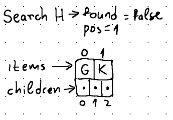
In all cases, the search() method also returns a boolean value indicating whether the search is successful or not.
This makes traversal quite easy, as if the boolean value evaluates to false, we can use the returned position to continue traversing the tree until we eventually find a data item with the desired key.
Consequently, we can search the entire tree as follows:
func (t *BTree) Find(key []byte) ([]byte, error) {
	for next := t.root; next != nil; {
		pos, found := next.search(key)

		if found {
			return next.items[pos].val, nil
		}

		next = next.children[pos]
	}

	return nil, errors.New("key not found")
}
btree.go
Inserting Data
Data insertion involves traversing the tree until we find a leaf node capable of accommodating our data item while still maintaining sorted order throughout the tree and keeping items within the boundaries set by minItems and maxItems.
Let's start by defining a helper method that allows us to insert a data item at any arbitrary position of a B-Tree node:
func (n *node) insertItemAt(pos int, i *item) {
	if pos < n.numItems {
		// Make space for insertion if we are not appending to the very end of the "items" array
		copy(n.items[pos+1:n.numItems+1], n.items[pos:n.numItems])
	}
	n.items[pos] = i
	n.numItems++
}
node.go
Naturally, reaching a leaf node doesn't guarantee that the node has enough capacity to accommodate our data item. It may already be full. In such cases we perform a transformation called "node split":
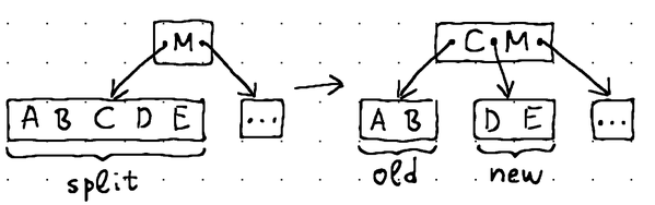
With a node split, we introduce a brand new node into the tree. We take the middle item out of the existing leaf node and move it up to its parent. We then take the second half of the data items from the existing leaf node and move them to the newly created node. Finally, we link the newly created node to the parent, inserting a new child pointer immediately after the middle item.
The need of rearranging children calls for adding another helper method to our node structure:
func (n *node) insertChildAt(pos int, c *node) {
	if pos < n.numChildren {
		// Make space for insertion if we are not appending to the very end of the "children" array.
		copy(n.children[pos+1:n.numChildren+1], n.children[pos:n.numChildren])
	}
	n.children[pos] = c
	n.numChildren++
}
node.go
Splitting the leaf node assumes that its parent has enough capacity to accommodate the middle item. However, the parent could easily be full as well, and we may face the same situation with its ancestors. Because of that, it's not unusual for node splits to propagate all the way up to the root of the tree. This requires careful consideration as we plan the implementation of the split() method.
What we can do is have our insertion code traverse the tree recursively while ensuring that each subsequent node along the way to our leaf has sufficient capacity to accommodate a new item (remember that node splits can propagate up to the root).
This means that we can perform a split as soon as we reach the parent of a child that is already full. Our split() method will create a new node and move all necessary data items and child pointers from the existing child node to the new node. It will also return the middle item from the existing child node so that we can move it to the parent node.
Here is the entire code for performing a split:
func (n *node) split() (*item, *node) {
	// Retrieve the middle item.
	mid := minItems
	midItem := n.items[mid]

	// Create a new node and copy half of the items from the current node to the new node.
	newNode := &node{}
	copy(newNode.items[:], n.items[mid+1:])
	newNode.numItems = minItems

	// If necessary, copy half of the child pointers from the current node to the new node.
	if !n.isLeaf() {
		copy(newNode.children[:], n.children[mid+1:])
		newNode.numChildren = minItems + 1
	}

	// Remove data items and child pointers from the current node that were moved to the new node.
	for i, l := mid, n.numItems; i < l; i++ {
		n.items[i] = nil
		n.numItems--

		if !n.isLeaf() {
			n.children[i+1] = nil
			n.numChildren--
		}
	}

	// Return the middle item and the newly created node, so we can link them to the parent.
	return midItem, newNode
}
node.go
You certainly noticed that in the code above we are also sometimes moving child pointers around. That's because the split operation may propagate up to the root, in which case we will be splitting non-leaf nodes. Splitting non-leaf nodes is not unusual. In such cases, we simply need to move half of the child pointers from the splitting child node to the newly created node.
The complete code for inserting a new item into the tree reads:
func (n *node) insert(item *item) bool {
	pos, found := n.search(item.key)

	// The data item already exists, so just update its value.
	if found {
		n.items[pos] = item
		return false
	}

	// We have reached a leaf node with sufficient capacity to accommodate insertion, so insert the new data item.
	if n.isLeaf() {
		n.insertItemAt(pos, item)
		return true
	}

	// If the next node along the path of traversal is already full, split it.
	if n.children[pos].numItems >= maxItems {
		midItem, newNode := n.children[pos].split()
		n.insertItemAt(pos, midItem)
		n.insertChildAt(pos+1, newNode)
		// We may need to change our direction after promoting the middle item to the parent, depending on its key.
		switch cmp := bytes.Compare(item.key, n.items[pos].key); {
		case cmp < 0:
			// The key we are looking for is still smaller than the key of the middle item that we took from the child,
			// so we can continue following the same direction.
		case cmp > 0:
			// The middle item that we took from the child has a key that is smaller than the one we are looking for,
			// so we need to change our direction.
			pos++
		default:
			// The middle item that we took from the child is the item we are searching for, so just update its value.
			n.items[pos] = item
			return true
		}

	}

	return n.children[pos].insert(item)
}
node.go
As you can see, the code expects a node to serve as its starting point. Logically, this node should be the tree root (i.e., we should start an insertion by calling tree.root.insert(item)). The algorithm will then start traversing the tree from its root, recursively calling the insert() method until it reaches a leaf node suitable for insertion. In case a data item with the given key already exists in the tree, we can simply update its value, rather than creating a brand new item.
We will encapsulate the initial tree.root.insert(item) call in a separate method that will be a part of our B-Tree structure. But before we get to that, it is worth explaining what needs to be done in case the root node itself is already full.
Splitting the root node is slightly different from splitting other nodes. When the root node is full, there is no parent to move the middle item to and no room to introduce a new sibling. Therefore, with root nodes, the split operation involves introducing a brand new root node to replace the existing root. The existing root then becomes the new root's left child. Simultaneously, we introduce another new node to play the role of the new root's right child. Half of the items from the existing root are moved to the new right child, while the middle item becomes the only data item in the newly introduced root node.
The code reads:
func (t *BTree) splitRoot() {
	newRoot := &node{}
	midItem, newNode := t.root.split()
	newRoot.insertItemAt(0, midItem)
	newRoot.insertChildAt(0, t.root)
	newRoot.insertChildAt(1, newNode)
	t.root = newRoot
}
btree.go
With that, we can conclude this section by adding a wrapper method to our B-Tree structure to facilitate the insertion:
func (t *BTree) Insert(key, val []byte) {
	i := &item{key, val}

	// The tree is empty, so initialize a new node.
	if t.root == nil {
		t.root = &node{}
	}

	// The tree root is full, so perform a split on the root.
	if t.root.numItems >= maxItems {
		t.splitRoot()
	}

	// Begin insertion.
	t.root.insert(i)
}
btree.go
Our B-Tree is now ready to store data.
Deleting Data
Compared to insertion, deletion requires a little more effort to implement, as there are many more potential transformations that may have to occur to keep the tree balanced.
Let's begin by adding another helper method to our node structure that allows us to remove a data item from any given position in the items array. For convenience, we will also return the removed item. This will come in handy later, when implementing the final deletion algorithm.
func (n *node) removeItemAt(pos int) *item {
	removedItem := n.items[pos]
	n.items[pos] = nil
	// Fill the gap, if the position we are removing from is not the very last occupied position in the "items" array.
	if lastPos := n.numItems - 1; pos < lastPos {
		copy(n.items[pos:lastPos], n.items[pos+1:lastPos+1])
		n.items[lastPos] = nil
	}
	n.numItems--

	return removedItem
}
node.go
There are two possibilities when deleting an item: it may be located at an internal node or at a leaf node. For leaf nodes, we can simply remove the item. However, with internal nodes, we must first find the item's inorder successor, swap it with the original item, and then take the inorder successor out of the leaf node where we found it.
In both cases, removing the item may result in an underflow at the leaf node. An underflow is the condition in which a node contains fewer items than the limit declared by minItems.
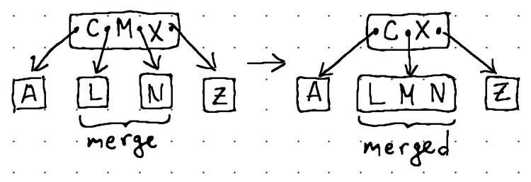
Underflows can be addressed by merging a node with its neighbor or by borrowing items from its adjacent siblings. Collectively, we call this operation a "node fill" (since we are filling the node with items, one way or another, in order to restore the limits set by minItems).
While borrow operations generally don't disrupt the balance of the tree, merge operations "steal" items from parent nodes and may therefore result in further underflows propagating up to the root of the tree. This is something important to keep in mind when designing the deletion algorithm.
In light of that fact, during a merge we will surely have to reorganize a node's children, so let's add another helper method to our node structure to make our implementation easier:
func (n *node) removeChildAt(pos int) *node {
	removedChild := n.children[pos]
	n.children[pos] = nil
	// Fill the gap, if the position we are removing from is not the very last occupied position in the "children" array.
	if lastPos := n.numChildren - 1; pos < lastPos {
		copy(n.children[pos:lastPos], n.children[pos+1:lastPos+1])
		n.children[lastPos] = nil
	}
	n.numChildren--

	return removedChild
}
node.go
Here's how the different fill operations look like in practice:
In terms of Go code, the borrow and merge operations can be expressed like this:
func (n *node) fillChildAt(pos int) {
switch {
// Borrow the right-most item from the left sibling if the left
// sibling exists and has more than the minimum number of items.
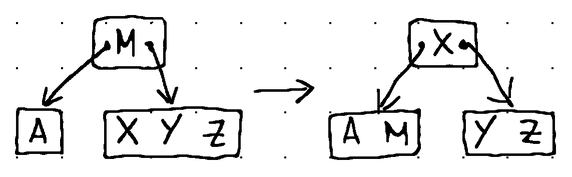
case pos > 0 && n.children[pos-1].numItems > minItems:
// Establish our left and right nodes.
left, right := n.children[pos-1], n.children[pos]
// Take the item from the parent and place it at the left-most position of the right node.
copy(right.items[1:right.numItems+1], right.items[:right.numItems])
right.items[0] = n.items[pos-1]
right.numItems++
// For non-leaf nodes, make the right-most child of the left node the new left-most child of the right node.
if !right.isLeaf() {
right.insertChildAt(0, left.removeChildAt(left.numChildren-1))
}
// Borrow the right-most item from the left node to replace the parent item.
n.items[pos-1] = left.removeItemAt(left.numItems - 1)
// Borrow the left-most item from the right sibling if the right
// sibling exists and has more than the minimum number of items.
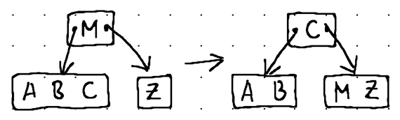
case pos < n.numChildren-1 && n.children[pos+1].numItems > minItems:
// Establish our left and right nodes.
left, right := n.children[pos], n.children[pos+1]
// Take the item from the parent and place it at the right-most position of the left node.
left.items[left.numItems] = n.items[pos]
left.numItems++
// For non-leaf nodes, make the left-most child of the right node the new right-most child of the left node.
if !left.isLeaf() {
left.insertChildAt(left.numChildren, right.removeChildAt(0))
}
// Borrow the left-most item from the right node to replace the parent item.
n.items[pos] = right.removeItemAt(0)
// There are no suitable nodes to borrow items from, so perform a merge.
default:
// If we are at the right-most child pointer, merge the node with its left sibling.
// In all other cases, we prefer to merge the node with its right sibling for simplicity.
if pos >= n.numItems {
pos = n.numItems - 1
}
// Establish our left and right nodes.
left, right := n.children[pos], n.children[pos+1]
// Borrow an item from the parent node and place it at the right-most available position of the left node.
left.items[left.numItems] = n.removeItemAt(pos)
left.numItems++
// Migrate all items from the right node to the left node.
copy(left.items[left.numItems:], right.items[:right.numItems])
left.numItems += right.numItems
// For non-leaf nodes, migrate all applicable children from the right node to the left node.
if !left.isLeaf() {
copy(left.children[left.numChildren:], right.children[:right.numChildren])
left.numChildren += right.numChildren
}
// Remove the child pointer from the parent to the right node and discard the right node.
n.removeChildAt(pos + 1)
right = nil
}
}node.go
The fillChildAt() method seems huge, but if you carefully read the comments, you should be able to gain a strong understanding of how the different types of fill operations work.
For the actual deletion, we traverse the tree recursively starting from its root, searching for a data item matching the key that we want to delete. We may find the key residing at either an internal node or a leaf node. For leaf nodes, we can just go ahead and remove the item. For internal nodes, however, we need to alter the path of traversal in order to locate the inorder successor (the inorder successor is the item having the smallest key in the right subtree that's greater than the key of the current item).
When we locate the inorder successor, we remove it from the leaf node that it resides at and then return it to the preceding call in the call stack so that it can be used to for replacing the original data item that we intended to delete.
As we traverse the tree back up from the leaf to the root, we check whether we have caused an underflow with our deletion or with any subsequent merges and perform the respective repairs.
The code looks like this:
func (n *node) delete(key []byte, isSeekingSuccessor bool) *item {
	pos, found := n.search(key)

	var next *node

	// We have found a node holding an item matching the supplied key.
	if found {
		// This is a leaf node, so we can simply remove the item.
		if n.isLeaf() {
			return n.removeItemAt(pos)
		}
		// This is not a leaf node, so we have to find the inorder successor.
		next, isSeekingSuccessor = n.children[pos+1], true
	} else {
		next = n.children[pos]
	}

	// We have reached the leaf node containing the inorder successor, so remove the successor from the leaf.
	if n.isLeaf() && isSeekingSuccessor {
		return n.removeItemAt(0)
	}

	// We were unable to find an item matching the given key. Don't do anything.
	if next == nil {
		return nil
	}

	// Continue traversing the tree to find an item matching the supplied key.
	deletedItem := next.delete(key, isSeekingSuccessor)

	// We found the inorder successor, and we are now back at the internal node containing the item
	// matching the supplied key. Therefore, we replace the item with its inorder successor, effectively
	// deleting the item from the tree.
	if found && isSeekingSuccessor {
		n.items[pos] = deletedItem
	}

	// Check if an underflow occurred after we deleted an item down the tree.
	if next.numItems < minItems {
		// Repair the underflow.
		if found && isSeekingSuccessor {
			n.fillChildAt(pos + 1)
		} else {
			n.fillChildAt(pos)
		}
	}

	// Propagate the deleted item back to the previous stack frame.
	return deletedItem
}
node.go
Similar to insertion, we extract the starting point of our deletion algorithm into a method attached directly to the B-Tree structure, which looks like this:
func (t *BTree) Delete(key []byte) bool {
	if t.root == nil {
		return false
	}
	deletedItem := t.root.delete(key, false)

	if t.root.numItems == 0 {
		if t.root.isLeaf() {
			t.root = nil
		} else {
			t.root = t.root.children[0]
		}
	}

	if deletedItem != nil {
		return true
	}
	return false
}
btree.go
We now have a fully working deletion procedure.
Conclusion
With this, we wrap up our article on B-Trees. As usual, the source code is available in our GitHub repository over here:
 cloudcentricdev
The repository also contains a convenient CLI with a B-Tree visualizer that will let you play around with the implementation interactively in order to solidify your understanding of B-Trees.
Here is a demo:
As always, I hope this post was informative and helpful. If you have any further questions or need clarification on anything discussed, feel free to reach out.
References
The following publications were referenced in the writing of this article:
- R. Beyer and E. McCreight. 1970. "Organization and Maintenance of Large Ordered Indices".
- D. Colmer. 1979. "The Ubiquitous B-Tree".
- D. Knuth. 1973. "The Art of Computer Programming, Volume 3: Sorting and Searching"
In addition, I referenced source code from the following Go-based B-Tree implementations:
- Pebble B-Tree by Cockroach Labs
- GoDS B-Tree by Emir Pasic